Today I ran a 12-hour simulation around Mount Fuji at 500 m resolution in the WOOF web app from Recast Systems, with boundary conditions from GFS 0.25°. I think the result is excellent: it ran on an RTX PRO 6000 (on-demand instance), took 11 minutes 40 seconds and cost 1.34 USD in total. Video demo below: https://blog-assets.ringsaturn.me/pic/2026/2026-10-10-recast-gpu-woof/recast-area-tsk-2026-10-10-1600gmt%2B9-mobile.mp4 This surprised me. It suggests that in the future, with higher-resolution real-time observations (satellite remote sensing in particular), rapid rolling corrections to the assimilation output of large-scale models, followed by a model like WOOF, a port of WRF-ARW to the GPU, could bring a large improvement to local weather forecasting and hazard warning, especially for severe convective weather. ...

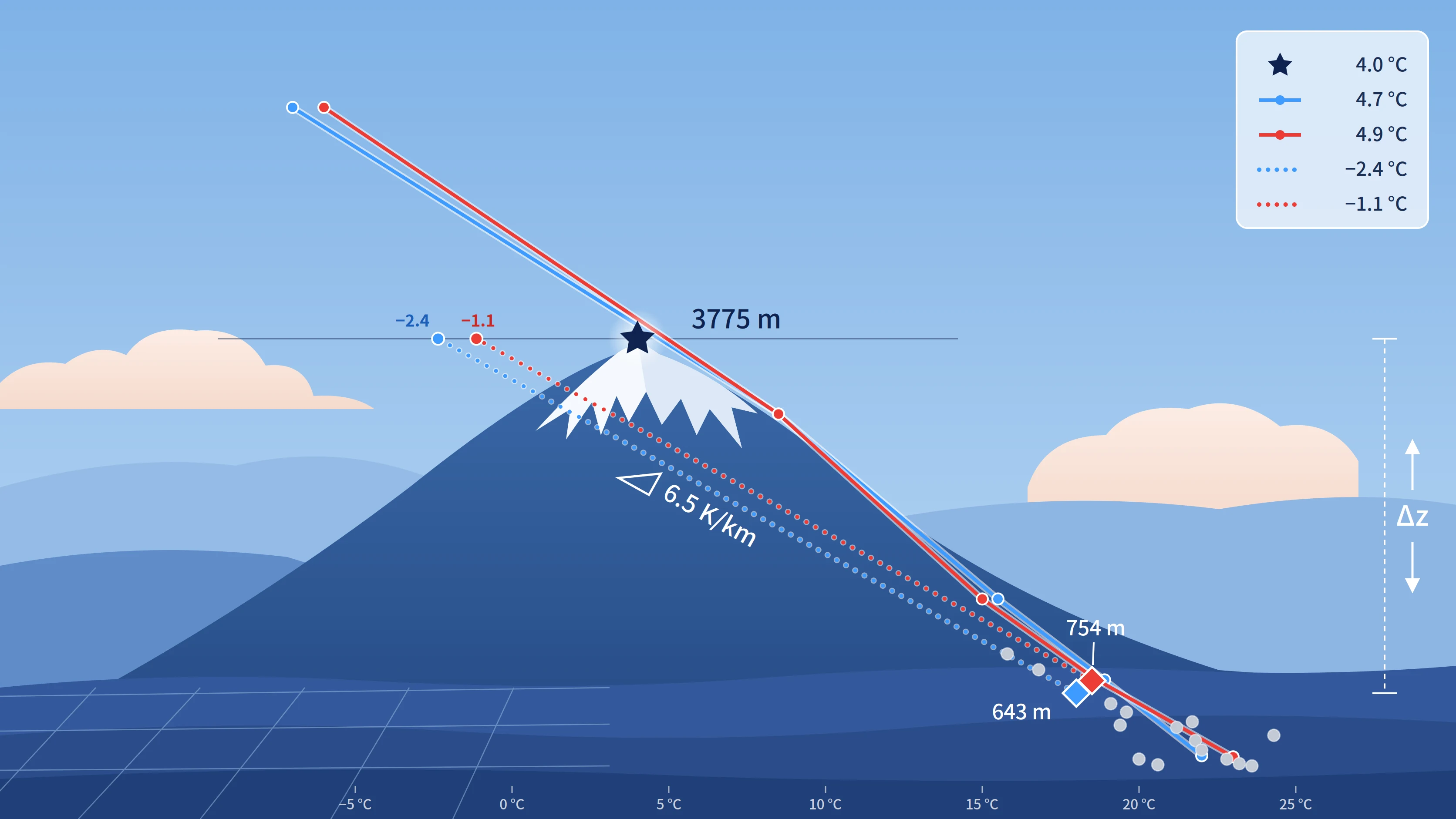
Verifying the 6.5 K/km elevation correction of GFS and ECMWF 2 m temperature against about 3000 stations over four seasons, and the pressure-level method with a decaying near-surface anomaly that xue now uses

In the previous post, 雪：更快速更流畅的气象数据动画 (Chinese), I packed forecast variables into a single-file container, .xue, which the browser read frame by frame through its index. For two variables of one GFS run, per-frame precolored PMTiles (zoom 0–4) came to 3,205.87 MB, the source GRIB2 was 137.73 MB, and .xue brought it down to about 65 MB. The size problem was solved. The problem with a custom container is that only its own decoder can read it. ...

Picking up where I left off: earlier this year I built a project called sitian, which analyzes weather processes from a sequence of synoptic charts over a period of time. Using it myself and backtesting it against historical weather, I found that combined analysis across multiple data sources did not work well. Take one example: a region is about to be affected by a typhoon, and the relevant data includes: Radiosonde soundings around the typhoon’s track Model forecast data Satellite observations Radar data Surface observations as supporting context The previous setup made it awkward to handle fairly complex combinations of input data. It also meant maintaining and integrating several data sources. So the sitian project has, in practice, stopped running. ...

ringsaturn/shachen The DEBRA algorithm (Miller et al. 2017, doi:10.1002/2017JD027365) is a method I have been following for a long time for identifying dust from satellite data. The unique aspect of this algorithm is its background estimation method, which avoids interference from special ground backgrounds such as deserts and lakebeds. Furthermore, the algorithm is designed for highly targeted engineering applications, aiming to be an all-weather recognition algorithm that provides users with fast, high-contrast output, bypassing the traditional need to introduce aerosol optical thickness.

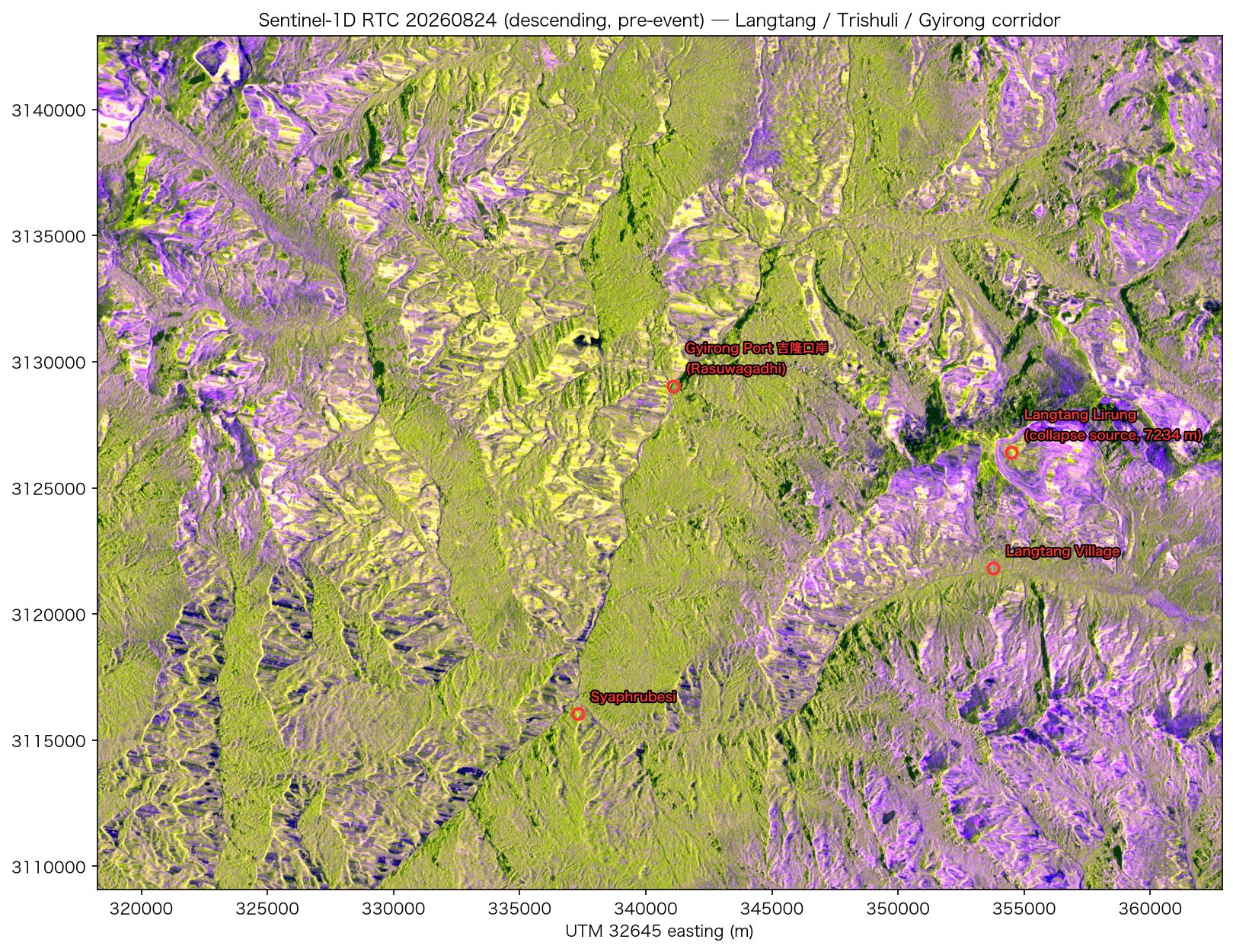
Note The satellite data in this post (Sentinel-1, NISAR and the optical scenes) was retrieved, processed and composited by the author. Claude compiled the text from those processed results and from public news reporting. Processing parameters and acquisition times are taken from the data itself; the event description and casualty figures come from the public sources linked in the text. At 02:52:10 UTC on 2026-08-26 (08:37 Nepal time, 10:52 China time), an ice and rock cliff on the north side of Langtang Lirung collapsed inside Langtang National Park. USGS located the source from seismic waves, on the north face of a peak roughly 7,200 m high; the main event released energy equivalent to M5.2, followed about 3 hours later by a secondary collapse equivalent to M4.2. AntarcticGlaciers gives the detachment coordinates as 28.2853°N, 85.5252°E and states that the present evidence does not support a glacial lake outburst flood (GLOF); the proposed mechanism is a multi-hazard cascade of ice and bedrock failure, rock/ice avalanche and debris flow, temporary river blockage, then outburst flooding. The author describes all of these as preliminary. The debris flow travelled about 100 km down the Bhote Koshi and Trishuli rivers and destroyed the customs facilities at the Rasuwagadhi border crossing along with the China–Nepal highway. The Wikipedia article records, as of 28 August, 547 dead and 977 missing on the Nepali side and 5 dead and 558 missing on the Chinese side; the search is ongoing, sources differ in what they count and when they were updated, and the figures are still changing. The same area saw a large ice and rock avalanche during the 2015 Gorkha earthquake that buried villages in the Langtang valley and killed more than 350 people. This post records the data work done in the two weeks after the event: building the Sentinel-1 pre-event baseline, processing the first obtainable post-event SAR data (NISAR, L-band) and the first post-event Sentinel-1 scene, and then the four viewing geometries that followed. ...

It has been a few years since the tzf project family was started. The last systematic look back at its development history was History of package tzf in early 2023. Since then, there have been various updates and maintenance work, mostly focused on non-core optimizations and supplementary features. In spring 2026, several long-pending important changes were finally completed: Introducing topology-aware processing to eliminate gaps and overlaps introduced during polygon simplification; Based on topology-aware processing, developing a more efficient data distribution format — ~17 MB for full-precision data and ~5.4 MB for simplified data; Introducing YStripes index acceleration, inspired by the tg project. Topology-Aware Processing The raw data is essentially a collection of polygons. Because the raw boundaries are highly detailed, the data volume is large, so polygon simplification is necessary. Many of these polygons share boundaries, but in the previous approach, each polygon was simplified independently using RDP. This caused a known issue that existed since the project’s early days: gaps appearing in areas that should be fully covered, and unwanted polygon overlaps introduced by simplification: ...

There is no built-in UV index in the original’s NOAA’s GFS data. However, Open Meteo provides UV index forecast in GFS’s data API and other weather models. That’s very interesting because it means that Open Meteo is doing some additional processing on top of the raw GFS data to derive the UV index. So I dig into it’s source code to see how they are calculating the UV index: 1 2 3 4 5 6 7 8 9 10 11 // https://github.com/open-meteo/open-meteo/blob/bf9577492dde460f9428d5d892b43bab9faa93ef/Sources/App/Gfs/GfsVariableDownloadable.swift#L473-L477 func multiplyAdd(domain: GfsDomain) -> (multiply: Float, add: Float)? { switch self { // ... case .uv_index, .uv_index_clear_sky: // UVB to etyhemally UV factor 18.9 https://link.springer.com/article/10.1039/b312985c // 0.025 m2/W to get the uv index // compared to https://www.aemet.es/es/eltiempo/prediccion/radiacionuv return (18.9 * 0.025, 0) // ... That make things simple. Just use existing GFS UVB data and apply a simple linear transformation to get the UV index.

A few days ago, I wanted to organize my resume information. Following my usual habit, I wrote it in LaTeX. However, when I wanted to publish it online to share the resume link, I needed to upload the PDF somewhere. The PDF file of the resume is a binary file, and I didn’t want to store it directly in the repository. So I decided to use GitHub Actions to automatically compile the LaTeX file and publish the generated PDF to GitHub Pages. ...