Creating Elevation RGB Tiles Around Mount Fuji

TLDR

A few days ago, while searching for information, I discovered MapTiler’s elevation profile visualization page, which works excellently:

This is really well done, and it’s entirely implemented in the browser https://t.co/R1vQMbdYAo pic.twitter.com/IyTYy5Fxo1
— ringsaturn.me (@ringsaturn_me) January 10, 2024

On their official blog, I found a 2019 post mentioning that the technique encodes elevation data into the RGB channels of an image and then decodes it in the browser. This allows elevation visualization directly in the browser—especially for continuous profile data—by downloading a few images to plot a continuous elevation curve.

On GitHub, I found the syncpoint/terrain-rgb project, which provides a complete guide for converting elevation data into RGB images.

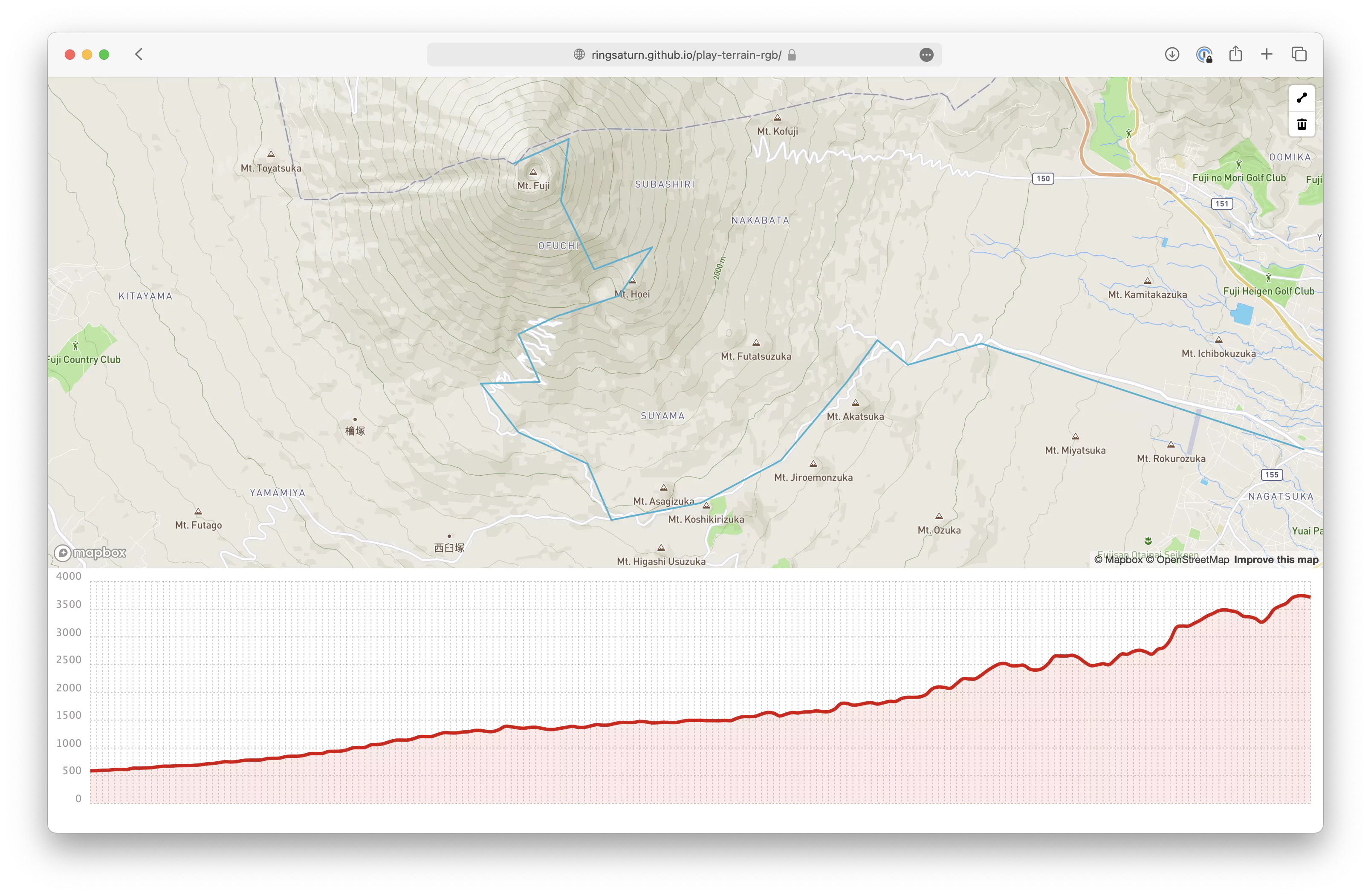
I placed my organized code into the ringsaturn/play-terrain-rgb repository. The workflow is identical to @syncpoint’s, with only minor parameter differences and source data variations.

I also modified the code from https://github.com/maptiler/samples/tree/main/cloud/elevation-profile to publish a visualization page for elevation data around Mount Fuji, with the following result:

Experience it here: https://ringsaturn.github.io/play-terrain-rgb

Workflow

I downloaded ASTER GDEM v3 data, which is a global 30m resolution elevation dataset. The download link is on the USGS website.

Since this is just a demo, I only used the file covering Mount Fuji: ASTGTMV003_N35E138_dem.tif.

According to the repository instructions, I needed a software environment capable of various geospatial data computations:

1
brew install gdal geoip libspatialite librasterlite spatialite-gui spatialite-tools

Subsequent data processing used many Python geospatial packages. For simplicity, I initialized a Python 3.11 environment with Conda:

1
conda create -n play-terrain-rgb python=3.11

Next, install dependencies. Unlike the original repository instructions, rasterio must be installed by building from source:

1
pip install rasterio --no-binary rasterio

Otherwise, rio will not find the rgbify CLI plugin.

Then install the remaining dependencies:

1
pip install rasterio rio-rgbify rio-mbtiles mbutil

You can inspect the original DEM file information with rio info:

1
rio info --indent 2 ASTGTMV003_N35E138_dem.tif

 1
 2
 3
 4
 5
 6
 7
 8
 9
10
11
12
13
14
15
16
17
18
19
20
21
22
23
24
25
26
27
28
29
{
  "blockxsize": 256,
  "blockysize": 256,
  "bounds": [
    137.999861111111, 34.99986111111112, 139.00013888888876, 36.0001388888889
  ],
  "colorinterp": ["gray"],
  "compress": "lzw",
  "count": 1,
  "crs": "EPSG:4326",
  "descriptions": ["Band 1"],
  "driver": "GTiff",
  "dtype": "int16",
  "height": 3601,
  "indexes": [1],
  "interleave": "band",
  "lnglat": [138.4999999999999, 35.500000000000014],
  "mask_flags": [["all_valid"]],
  "nodata": null,
  "res": [0.000277777777777778, 0.000277777777777778],
  "shape": [3601, 3601],
  "tiled": true,
  "transform": [
    0.000277777777777778, 0.0, 137.999861111111, 0.0, -0.000277777777777778,
    36.0001388888889, 0.0, 0.0, 1.0
  ],
  "units": [null],
  "width": 3601
}

Because the original coverage area is too large, I only needed the data around Mount Fuji. Therefore, I clipped it first:

1
gdal_translate -projwin 138.626942 35.439672 138.899882 35.255449 ASTGTMV003_N35E138_dem.tif ASTGTMV003_N35E138_dem_clip.tif

Next, reproject the file to Web Mercator so it can be displayed in the browser:

1
gdalwarp -t_srs EPSG:3857 -dstnodata None -novshiftgrid -co TILED=YES -co COMPRESS=DEFLATE -co BIGTIFF=IF_NEEDED -r lanczos ASTGTMV003_N35E138_dem_clip.tif ASTGTMV003_N35E138_dem_clip_EPSG3857.tif

1
2
Creating output file that is 914P x 756L.
Processing ASTGTMV003_N35E138_dem_clip.tif [1/1] : 0...10...20...30...40...50...60...70...80...90...100 - done.

Inspect the reprojected file’s information:

1
rio info --indent 2 ASTGTMV003_N35E138_dem_clip_EPSG3857.tif

 1
 2
 3
 4
 5
 6
 7
 8
 9
10
11
12
13
14
15
16
17
18
19
20
21
22
23
24
25
26
27
28
29
{
  "blockxsize": 256,
  "blockysize": 256,
  "bounds": [
    15431865.404742576, 4198669.725048377, 15462269.950626153, 4223818.342868929
  ],
  "colorinterp": ["gray"],
  "compress": "deflate",
  "count": 1,
  "crs": "EPSG:3857",
  "descriptions": ["Band 1"],
  "driver": "GTiff",
  "dtype": "int16",
  "height": 756,
  "indexes": [1],
  "interleave": "band",
  "lnglat": [138.76336989692504, 35.347779733715655],
  "mask_flags": [["all_valid"]],
  "nodata": null,
  "res": [33.265367487502644, 33.265367487502644],
  "shape": [756, 914],
  "tiled": true,
  "transform": [
    33.265367487502644, 0.0, 15431865.404742576, 0.0, -33.265367487502644,
    4223818.342868929, 0.0, 0.0, 1.0
  ],
  "units": [null],
  "width": 914
}

Then use rio rgbify to convert the elevation data into an RGB image:

1
rio rgbify -b -10000 -i 0.001 ASTGTMV003_N35E138_dem_clip_EPSG3857.tif ASTGTMV003_N35E138_dem_clip_EPSG3857.RGB.tif

The output image looks roughly like this:

We can query the original file’s elevation at a target latitude and longitude:

1
gdallocationinfo -wgs84 ASTGTMV003_N35E138_dem.tif 138.72739076614383 35.36067113569001

1
2
3
4
Report:
  Location: (2619P,2302L)
  Band 1:
    Value: 3756

Then query the converted RGB file:

1
gdallocationinfo -wgs84 ASTGTMV003_N35E138_dem_clip_EPSG3857.RGB.tif 138.72739076614383 35.36067113569001

1
2
3
4
5
6
7
8
Report:
  Location: (336P,325L)
  Band 1:
    Value: 209
  Band 2:
    Value: 234
  Band 3:
    Value: 72

The three values read are 209, 234, and 72. Using the conversion formula:

$$ \mathit{height} = -10000 + \bigl((R \times 256 \times 256 + G \times 256 + B) \times 0.001\bigr) $$

(where 0.001 is from the -i parameter passed to rio rgbify), we can compute:

1
2
height = -10000 + ((209 * 256 * 256 + 234 * 256 + 72) * 0.001)
# 3757

The error is acceptable.

Next, to display on a map, we need to convert the RGB image into tiles. I used the gdal2tiles.py tool:

1
time gdal2tiles.py --zoom=5-19 --processes=16 ASTGTMV003_N35E138_dem_clip_EPSG3857.RGB.tif ./tiles

1
2
3
4
5
Generating Base Tiles:
...10...20...30...40...50...60...70...80...90...100 - done.
Generating Overview Tiles:
0...10...20...30...40...50...60...70...80...90...100 - done.
gdal2tiles.py --zoom=5-19 --processes=16  ./tiles  1332.07s user 360.34s system 1297% cpu 2:10.39 total

Note: If you regenerate tiles multiple times, gdal2tiles.py will modify the zoom range in the generated HTML, so you may need to manually adjust it depending on your situation.

Finally, we can convert the tiles into MBTiles format using mb-util:

1
mb-util --image_format=png --scheme=tms ./tiles/ ./ASTGTMV003_N35E138_dem_clip_EPSG3857.RGB.mbtiles

1
2
176000 tiles inserted (24076 tiles/sec)
mb-util --image_format=png --scheme=tms ./tiles/   2.12s user 3.92s system 75% cpu 7.995 total

TLDR#

Workflow#

TLDR

Workflow