The full name of the GHCNd dataset is the Global Historical Climatology Network daily. It is a global observation dataset publicly released by NOAA, with data starting from 1763, containing daily meteorological observation data from a total of 120,000 weather stations worldwide. The monthly summary version of the GHCNd dataset is the Global Historical Climatology Network monthly.
During the weekend, I performed some statistical analysis on this dataset, and I’d like to record the general processing workflow.
First, I synchronized the data. This dataset is stored on NOAA’s own servers as well as on AWS/GCP public datasets. For simplicity, I chose the dataset on AWS. Initially, I used AWS CLI for synchronization, but JuiceFS can also be used.
| |
Subsequently, I performed daily and monthly level data statistical work.
The core approach involves using Polars to calculate the required statistical information within specified time ranges. For example, the daily statistics calculation:
| |
Then I used Matplotlib for visualization:
| Daily Data | Monthly Data | |
|---|---|---|
| Beijing |  |  |
| Shanghai |  |  |
| Tokyo |  |  |
The processing code is open-sourced on GitHub at ringsaturn/ghcn-showcases. Additionally, a static page displaying statistical information for select stations is available on GitHub Pages at ghcn-showcases.
Web Page Preview:
Beijing Display Preview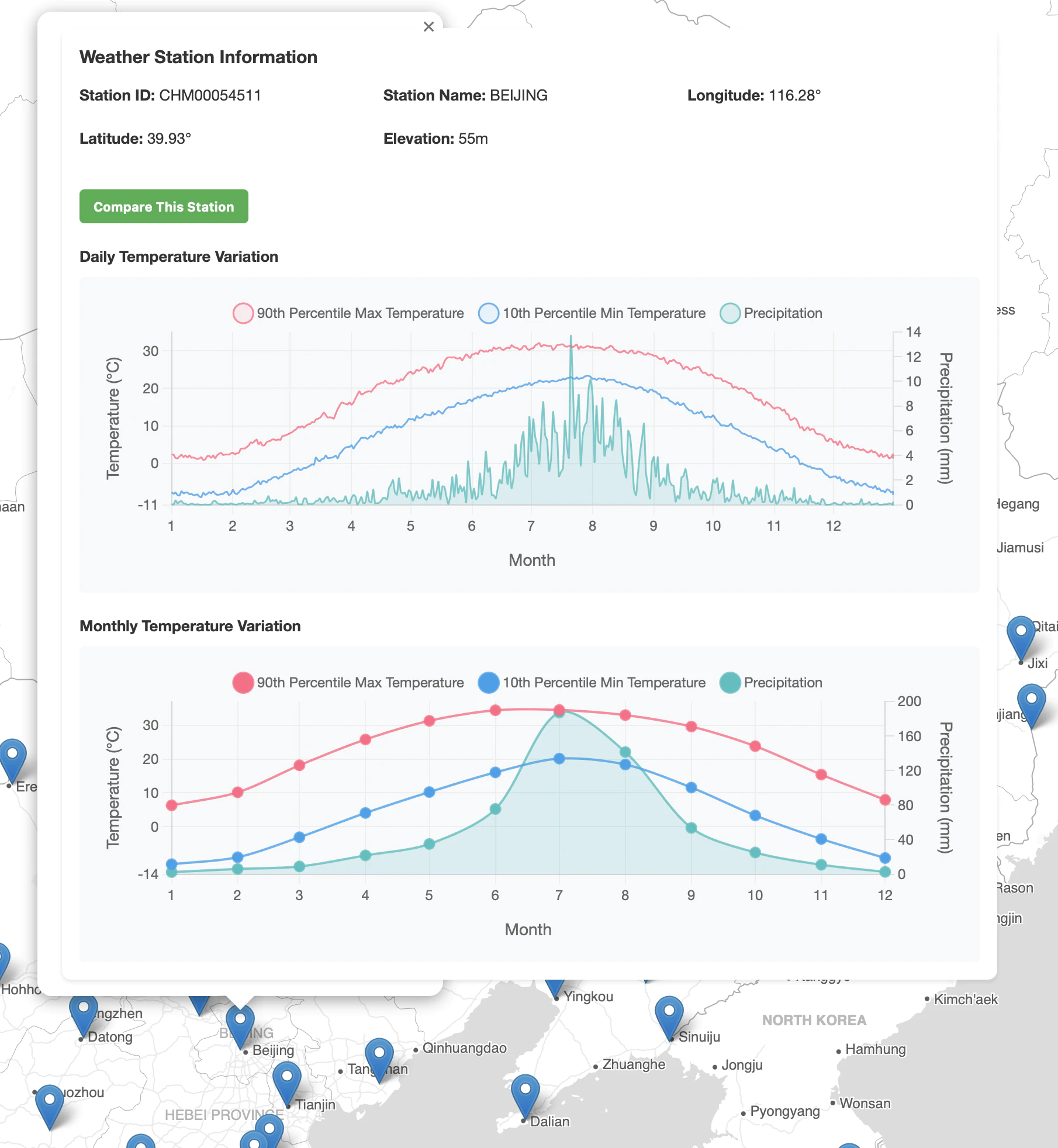
Shanghai Display Preview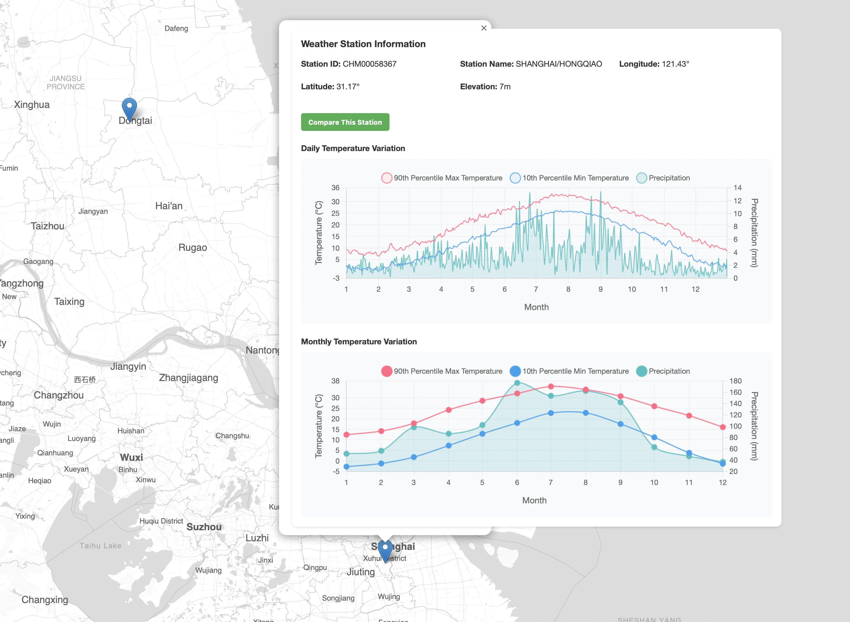
Temperature Comparison of Beijing/Shanghai/Tokyo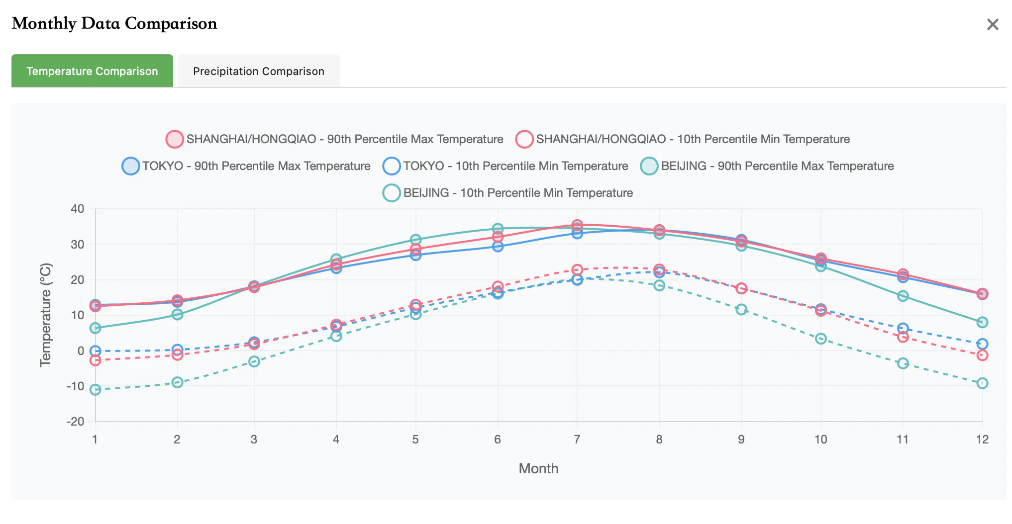
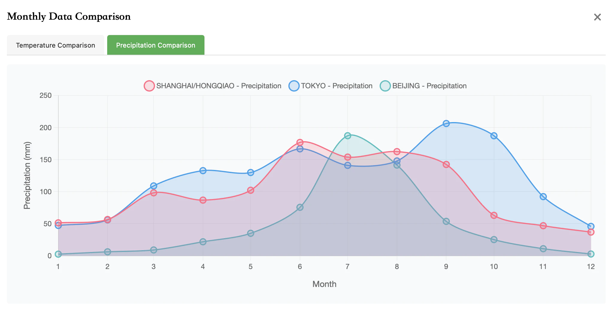
Precipitation Comparison of Beijing/Shanghai/Tokyo